[R][Statistics]Time Series Analysis with S&P 500 Stock price

I have not been writing statistical/ ML blog posts for a while. So, it’s good to come back!

Today, I will demonstrate how to apply time series analysis on forecasting stock market price. I won’t go over deep theory of time series analysis but will show the most fundamental model of time series analysis model.

 

 

1. Open the libraries that we need. Then, open the data. 

2. Exploring the data

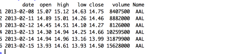
Here are the first 6 rows of the data. It contains date, open, high, low,close price and volume. The last variable indicates the initial of stock market. In this example, AAL is American Airlines Group.

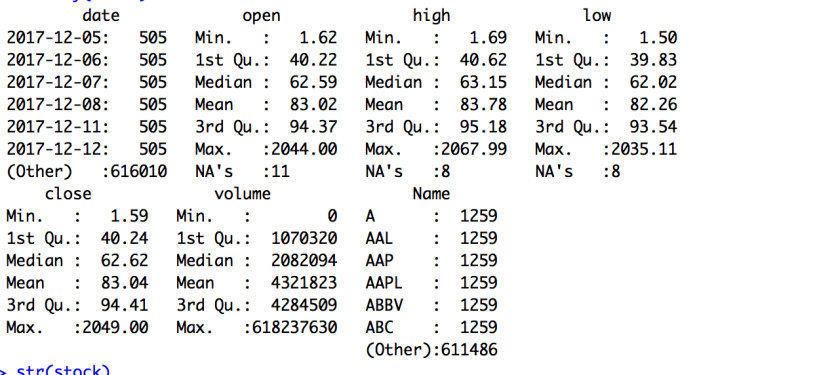
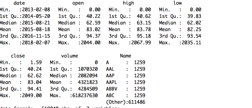
By using summary command, it’s easy way to get an overview of the data. In this case, there are a few NA values in price variables. Getting rid of NA values would make data handling easier.

The prices approximately ranges from 1.5 to 2067 while the median values are around 62-63. It indicates that the price distribution is likely to be skewed. We can check it visually soon.

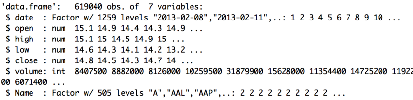
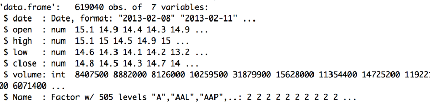
By using str command, we can check each variable’s format. We can see that date variable is treated as a factor variable. It would be better to change the data variable into date format.

3. Data Cleaning

From the previous step, 1. there are NA values that we want to discard, 2. transforming the date variable format.

Just getting rid of them would cause the difference in each variable length.The good news is that there were not many NA values in each price variable. Simply, we can change NA value to 0. 

Then, we had trouble with the format of data variable. We can change it into the right format by using as.Date command.

Let’s double check how the data is altered.

Now, there are no NA values. Instead, the minimum values are all 0 across open, high,low and volume. Date variable is now in proper date format.

4. Histogram-Check the distribution of price variables

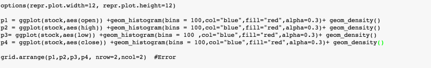
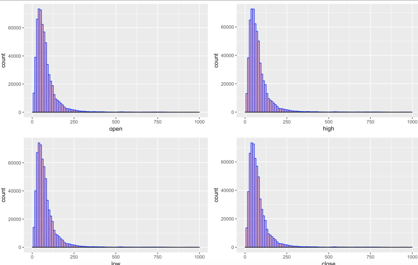
The price distributions are quite similar to each other. As we expected, the distributions are kind of right skewed which means the median is lower than the mean values.

5. Time Series Analysis Model- A bit of Theory

The most basic time series models are AR,MA and ARMA model.

AR(Auto Regressive Model)

Autoregressive (AR) models are models where the value of variable in one period is related to the values in the previous period. In other words, Autoregression is a time series model that uses observations from previous time steps as input to a regression equation to predict the value at the next time step.  AR(p) is a Autoregressive model with p lags.

MA(Moving Average Model)

Moving average (MA) model accounts for the possibility of a relationship between a variable and the residual from the previous period. MA(q) is a Moving Average model with q lags.

The role of the random shocks in the MA model differs from their role in the autoregressive (AR) model in two ways. First, they are propagated to future values of the time series directly. Second, in the MA model, a shock affects X values only for the current period and q periods into the future; In contrast, in the AR model, a shock affects X values infinitely far into the future

ARMA

ARMA is the combined version between AR and MA.  The AR part involves regressing the variable on its own lagged (i.e., past) values. The MA part involves modeling the error term as a linear combination of error terms occurring contemporaneously and at various times in the past. It’s denoted as ARMA(p,q).

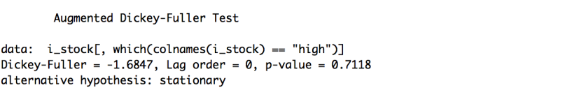
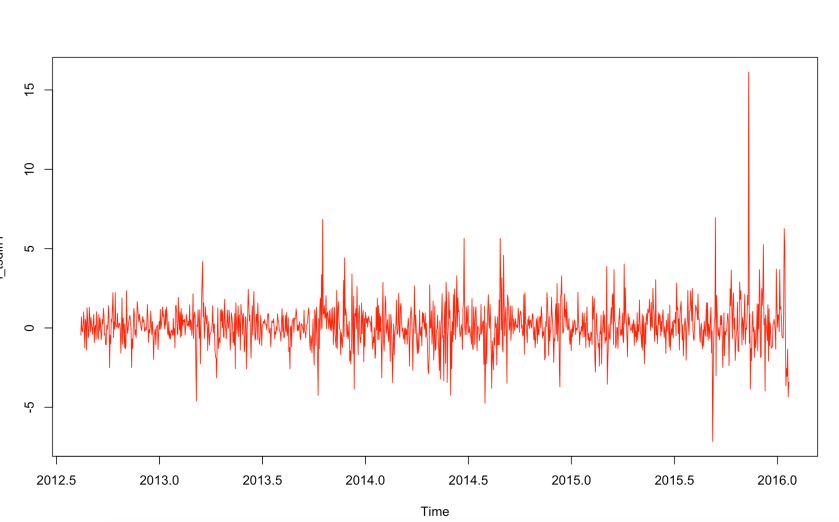
Assumption for these models:  The variance is constant while the mean fluctuates

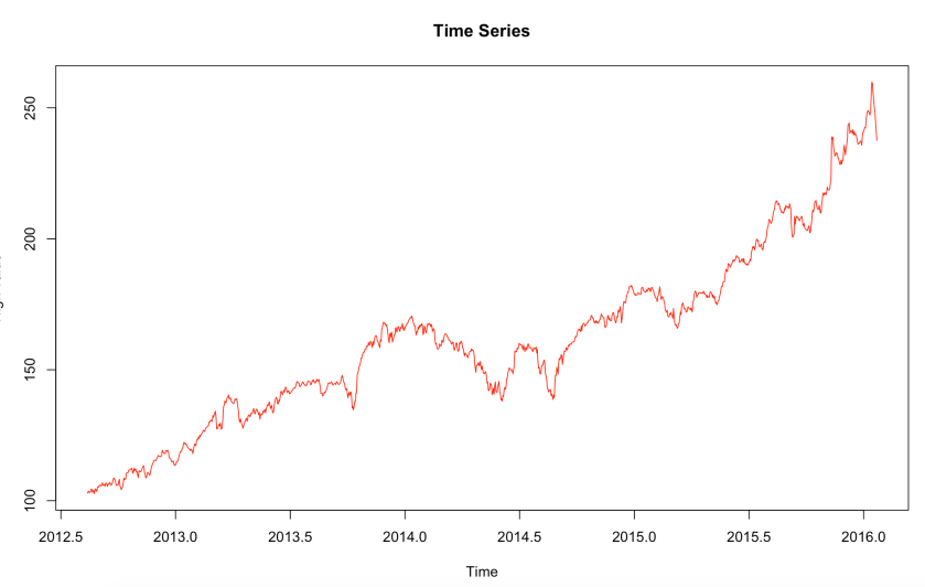
6. Create the function that creates time series object and Plot it

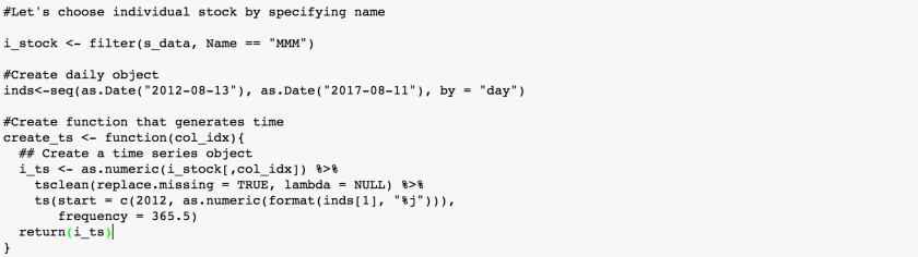
tsclean() is a convenient method for outlier removal and inputing missing values

ts() is used to create time-series objects

In this example, I used 3M stock(MMM) . Recently, the stock price plunged right after the most recent earning call.

7. Stationarity- A little bit of more theory

A stationary process has a mean and variance that do not change overtime and the process does not have trend. It’s a common assumption in many time series techniques is that the data are stationary.

But this time series does not look stationary. To confirm that we will use “Dickey-Fuller test” to determine stationarity.

In general sense,when the p value is smaller than 0.05, we can reject the null hypothesis. Since the p value is much higher than 0.05, we can’t reject the null hypothesis. In plain English, the series not stationary.

8.Differencing in time series

Differencing is a common solution used to make the variable stationary. Think about the concept of differentiation in basic calculus class.

 After applying differencing, it looks much more stationary.

9. Select Candidate Model

In the step 5,  I mentioned the three time series model: AR(p),MA(q) and ARMA(p,q). Now this step will discuss which model to select and which lag(p or q) to pick. The most popular way to decide which model to use is examining ACF and PACF plot which are autocorrelation function and partial autocorrelation function.

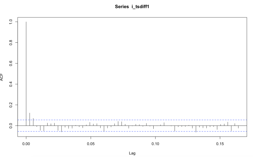
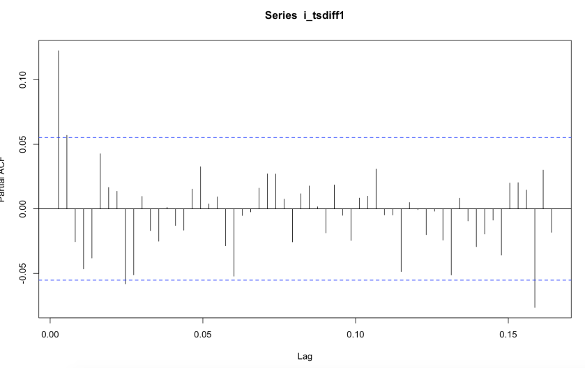
The blue line above shows significantly different values than zero. Clearly, the first graph above has a cut off on PACF curve after the 2nd lag or the 3rd lag which means this is mostly an AR(2)/AR(3) process.  The second graph above has a cut off on ACF curve after the 1st or 2nd lag which means it will be MA(1) or MA(2). But at the right side of the graph, there is a lag above blue line. So, let’s try to use another method of selecting candidate.

R has function that automatically chooses the most suitable ARIMA model.

 

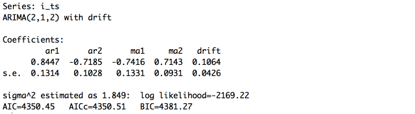
According to the result, ARIMA(2,1,2) would work the best.

 

10. Forecasting

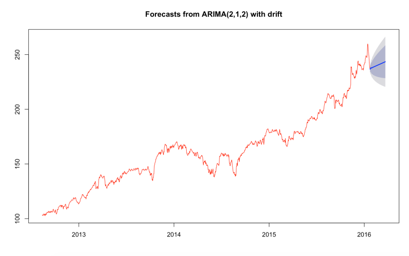
At least, the forecasting said the stock market price of 3M is likely to be increasing. So, good news for 3M investors!

 

Potential Next part

Using Recurrent Neural Network