

I was so pleased that so many people read my first statistical blog post: “which u.s. state does produce the most beer?”.
So, I decided to write another one. For this blog post, I worked on pokemon dataset from Kaggle.
Before talking about random forest ,which is one of the most popular machine learning methods,I will begin with corrleation plot. It’s like an appetizer before the main course.
Brief Idea of the dataset
Last time, I felt bad that I forgot to give a brief idea of the data. From now on, I will make sure to provide how the data looks like for each post.
Here is the snapshot of the head of the dataset. This dataset has total 13 variables with 800 pokemons.

- Number: ID for each pokemon
- Name: Name of each pokemon
- Type 1: Each pokemon has a type, this determines weakness/resistance to attacks
- Type 2: Some pokemon are dual type and have 2
- Total: sum of all stats that come after this, a general guide to how strong a pokemon is
- HP: hit points, or health, defines how much damage a pokemon can withstand before fainting
- Attack: the base modifier for normal attacks (eg. Scratch, Punch)
- Defense: the base damage resistance against normal attacks
- SP Atk: special attack, the base modifier for special attacks (e.g. fire blast, bubble beam)
- SP Def: the base damage resistance against special attacks
- Speed: determines which pokemon attacks first each round
Correlation Plot
R has a “corrplot” package and it offers great quality of visualzition on correlation analysis.
Since correlation analysis is for numerical variables, let’s separate variables into categorical and numerical.


Result

Simple,isn’t it? Now when you have a simple statistical report homework or work to submit, you can use this library and simply use “corrplot” function.It looks like total variable(dependent variable) is quite correlated with the rest of the variables. Interestingly, speed is not so related with defense skill but slightly related with special defense.
Random Forest
I know this concept might be new to many readers for this post. But let me try to explain this concept as simple as possible.

<Image: decision tree from https://www.edureka.co/blog/decision-trees/>
I think many of you have seen this tree. This is called decision tree. If you understand this, you are on the half way of understanding random forest. There are two keywords here – random and forests. Random forest is a collection of many decision trees. Instead of relying on a single decision tree, you build many decision trees say 100 of them. And you know what a collection of trees is called – a forest. And for higher accuracy, it’s randomized.
Let’s begin!
Step 1: Divide the dataset into training set and test set (for Cross validation).
The first step is randomly select “k” features from total “m” features.

In this example, I randomly assigned 70% of the data as “training” set while the rest of the data is assigned as “test” set. This procedure is called “Cross Validation“.
Then, what is Cross Validation?

<Image: Cross Validation from https://www.edureka.co/blog/implementation-of-decision-tree>
This image is quite self explanatory but let me elaborate. The example is 5- fold cross validation. For each fold, the each test set doesn’t duplicate to another. Using measurement metric(e.g. Mean Absolute Error, Root Suared Mean Error) , it averages the final measure of performance for each fold. By cross validation, it ensures randomization.
Step 2: Build the random forest model


Luckily, R is an open source so there are a lot of packages that make people life easier. Random Forest package provides randomForest function that enables to build random forest model so easily. After building the model on the train dataset, test the prediction on the test dataset.
Step 3: Variable Importance

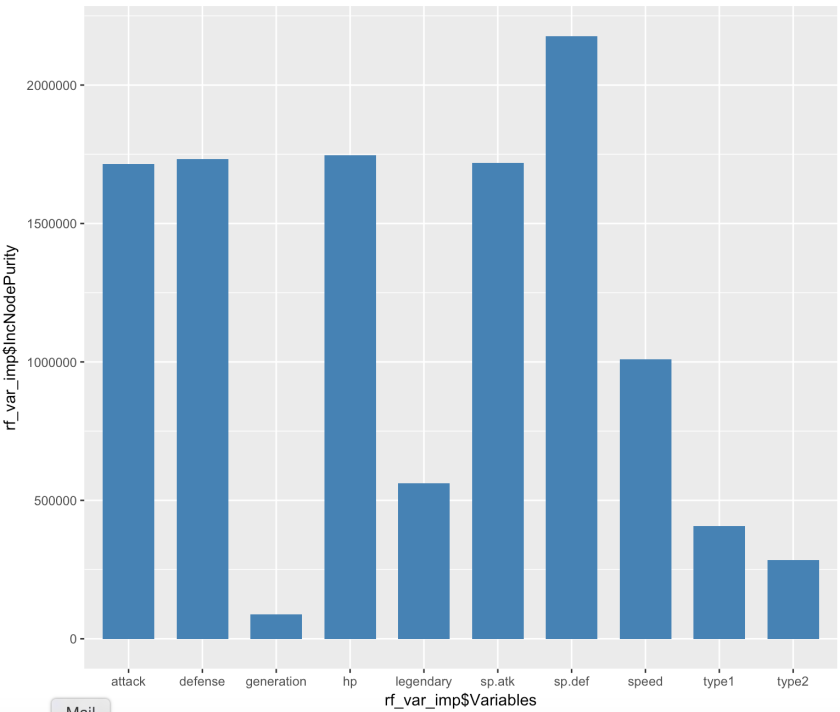
After building the random forest model, you can examine variable importance for the model. Again, I’m using ggplot to create nicer looking graphs. We can see that generation is the least important while special defense is the most significant in the model.
Step 4: Examine how the model is performing
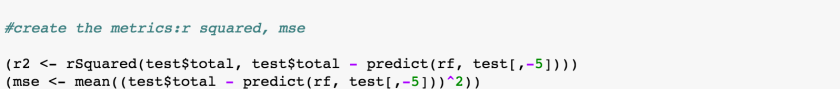

I’m using the two measurements in here: R-squared and MSE. R squared indicates how close the data are to the fitted regression line and MSE is the squared difference between the estimator and what is estimated. In short, the higher R-squared and lower MSE make the better model.

As a result, R squared is 0.93 and MSE is 994.81. It means that the model explains 93% of the variability of the response data around its mean.
I hope you guys enjoyed reading this!
Data Source: https://www.kaggle.com/abcsds/pokemon
